2. Google ColabでscRNA-seq解析
Google ColabはGoogleが提供するクラウドサービスで、対応しているのはPythonのみですが、無料でGPUを使うことができるのが魅力です。お手軽に深層学習を試してみたい場合には重宝します。 実行した設定は保存されないため、毎回ライブラリをインストールする必要がありますが、一般的なデータ解析ライブラリ群(行列演算や機械学習など)は既にインストールされているので、インストールの手間はそれほどないでしょう。
(2021/4/30追記:現在はRにも対応しています。 Google ColaboratoryでR言語を使う)
Python,Google Colaboratoryについては様々な参考資料や解説サイトがあります.例えば,以下のような資料も参考にしてください.
ここではPythonとGoogle Colabに慣れるため、データ読み込みと正規化、次元削減までを一般的なライブラリのみを用いて実行してみましょう。
参考: Jupyter と Google Colab との違い
HTMLブラウザ上で逐次的にコマンドを実行していくこれらのサービスがJupyter notebook (JupyterLab) です。Jupyter上で行う作業は自分のPC上で行うことになり、解析環境は自分のPCのマシンスペックに依存します。また、Dockerから起動することで、今回のシングルセルツール導入済み環境など、自由な解析環境を作ることができます。
Google Colab は Google社によって提供されている特殊なJupyter環境であり、Google クラウドにアクセスしている状態になります。そのため解析環境は手元のPCに依存しませんし、GPUを利用することも可能です。一方、Dockerなどを利用することはできず、Googleから提供されている環境のみ利用可能です。そのため環境にインストールされていないライブラリは毎回インストールし直す必要があり、大規模な解析環境構築には不向きです。
2.1. 推奨ブラウザ環境
Google Colaboratory は主要なブラウザはサポートしています.特にChromeとFirefoxでは完全に動作するよう検証されています.
以降の作業は全てGoogle Colab上で行います。
2.2. データ読み込み
wgetを使ってサンプルデータをダウンロードします。データサイズは5MBです。 これはPBMCの10種類の細胞を各500細胞ずつ使った5,000細胞のラベルありデータです。コンマで区切られたテキストファイル(csv形式)です。
[1]:
# ライブラリ読み込み(下記のライブラリは全てGoogle Colabにインストール済です)
import numpy as np
import pandas as pd
from matplotlib import pyplot as plt
from sklearn.manifold import TSNE
from sklearn.decomposition import PCA
import matplotlib.cm as cm
import seaborn as sns
%matplotlib inline
[2]:
# csvファイルをwgetでダウンロード
!wget http://nakatolab.iqb.u-tokyo.ac.jp/supplement/PBMC_10cell_types_total_500.csv.gz
--2021-04-30 12:22:13--  http://nakatolab.iqb.u-tokyo.ac.jp/supplement/PBMC_10cell_types_total_500.csv.gz
Resolving nakatolab.iqb.u-tokyo.ac.jp (nakatolab.iqb.u-tokyo.ac.jp)... 163.43.80.77
Connecting to nakatolab.iqb.u-tokyo.ac.jp (nakatolab.iqb.u-tokyo.ac.jp)|163.43.80.77|:80... connected.
HTTP request sent, awaiting response... 200 OK
Length: 5434256 (5.2M) [application/x-gzip]
Saving to: ‘PBMC_10cell_types_total_500.csv.gz.1’

PBMC_10cell_types_t 100%[===================>]   5.18M  1.68MB/s    in 3.1s

2021-04-30 12:22:17 (1.68 MB/s) - ‘PBMC_10cell_types_total_500.csv.gz.1’ saved [5434256/5434256]
[3]:
input_data = pd.read_csv("PBMC_10cell_types_total_500.csv.gz", index_col=0)
input_data.shape
[3]:
(32738, 5000)
[4]:
input_data.head()
[4]:
| ACAGTCGAGTTACG-1 | CACAATCTAAGGGC-1 | TATACCACGCTATG-1 | GTGTAGTGTCTATC-1 | TGCTATACGTATCG-1 | GCAGGCACTGCACA-1 | AGCGGCTGACAGTC-1 | CGAAGTACACTAGC-1 | TAACATGACCTCGT-1 | AACCGCCTCGAGAG-1 | TACGGCCTCACAAC-1 | GGCACGTGGCGGAA-1 | ACCGTGCTAGCGTT-1 | AGAAACGAACGTTG-1 | GCGGGACTTGCTTT-1 | AACGTGTGAGCGGA-1 | CGTGTAGAAACAGA-1 | AAGGTCTGATTCGG-1 | AGAGTGCTGCGTTA-1 | GTTCATACCCCTCA-1 | TATCTTCTCCTTAT-1 | GAGCGCTGGGAGGT-1 | CAGATGACAAGAAC-1 | AGAGGTCTTGCCAA-1 | ATGCCGCTACGTTG-1 | ATGCCGCTCCTCAC-1 | CGGGACTGCGTTGA-1 | CACCACTGCATCAG-1 | TAGTGGTGTGGATC-1 | GTTATGCTCCGTTC-1 | TATGGTCTTGCTGA-1 | GTGACCCTGTTCAG-1 | TTGAATGAAGGGTG-1 | TCCATAACTATTCC-1 | GTCGACCTTTTCAC-1 | CTAACACTAGTACC-1 | CAGGAACTCTCATT-1 | CTTTAGTGTTTCGT-1 | ATCAACCTGTCTTT-1 | TATTGCTGCTAGCA-1 | ... | ATCGGAACGGGAGT-1 | AGACTTCTCTAGAC-1 | TGCACGCTACCAGT-1 | TGGTTACTACTCAG-1 | CACGAAACGTACAC-1 | CCTATTGAGATAGA-1 | CCAGTCTGCCCTTG-1 | AACGTTCTATGCTG-1 | ACCCAAGACAGAGG-1 | GGAAGGACCTTAGG-1 | CAGAGGGACTACGA-1 | TGATACCTCAGAGG-1 | GCGATATGAATCGC-1 | TAGAGCACTGGTTG-1 | TACCATTGGAATCC-1 | ACGAGGGATCGTAG-1 | CTGAAGACCGATAC-1 | CAAGGACTACTTTC-1 | GTAGCATGGAATGA-1 | CGCAGGTGATTTCC-1 | GCGGCAACACCTGA-1 | TAGGCATGGACGAG-1 | TATGGGTGCAGAGG-1 | TGTCTAACCTGTCC-1 | AGTGTGACAAGCCT-1 | ACGGCGTGTGACCA-1 | ACACCCTGCGAACT-1 | ACACATCTTGGTTG-1 | GACTTTACCTGCTC-1 | AAACTTGAGCCTTC-1 | GAGTAAGACTAGTG-1 | ACCTGGCTATTCGG-1 | GTGAGGGAAAAGTG-1 | CTCTAATGTGGGAG-1 | GAGCAGGATCAGGT-1 | AATCTCTGAAGAAC-1 | ACGACCCTGCAGAG-1 | TATGGTCTCAAAGA-1 | TCTTGATGATCACG-1 | ACTGAGACTTCACT-1 | |
|---|---|---|---|---|---|---|---|---|---|---|---|---|---|---|---|---|---|---|---|---|---|---|---|---|---|---|---|---|---|---|---|---|---|---|---|---|---|---|---|---|---|---|---|---|---|---|---|---|---|---|---|---|---|---|---|---|---|---|---|---|---|---|---|---|---|---|---|---|---|---|---|---|---|---|---|---|---|---|---|---|---|
| 0 | 0.0 | 0.0 | 0.0 | 0.0 | 0.0 | 0.0 | 0.0 | 0.0 | 0.0 | 0.0 | 0.0 | 0.0 | 0.0 | 0.0 | 0.0 | 0.0 | 0.0 | 0.0 | 0.0 | 0.0 | 0.0 | 0.0 | 0.0 | 0.0 | 0.0 | 0.0 | 0.0 | 0.0 | 0.0 | 0.0 | 0.0 | 0.0 | 0.0 | 0.0 | 0.0 | 0.0 | 0.0 | 0.0 | 0.0 | 0.0 | ... | 0.0 | 0.0 | 0.0 | 0.0 | 0.0 | 0.0 | 0.0 | 0.0 | 0.0 | 0.0 | 0.0 | 0.0 | 0.0 | 0.0 | 0.0 | 0.0 | 0.0 | 0.0 | 0.0 | 0.0 | 0.0 | 0.0 | 0.0 | 0.0 | 0.0 | 0.0 | 0.0 | 0.0 | 0.0 | 0.0 | 0.0 | 0.0 | 0.0 | 0.0 | 0.0 | 0.0 | 0.0 | 0.0 | 0.0 | 0.0 |
| 1 | 0.0 | 0.0 | 0.0 | 0.0 | 0.0 | 0.0 | 0.0 | 0.0 | 0.0 | 0.0 | 0.0 | 0.0 | 0.0 | 0.0 | 0.0 | 0.0 | 0.0 | 0.0 | 0.0 | 0.0 | 0.0 | 0.0 | 0.0 | 0.0 | 0.0 | 0.0 | 0.0 | 0.0 | 0.0 | 0.0 | 0.0 | 0.0 | 0.0 | 0.0 | 0.0 | 0.0 | 0.0 | 0.0 | 0.0 | 0.0 | ... | 0.0 | 0.0 | 0.0 | 0.0 | 0.0 | 0.0 | 0.0 | 0.0 | 0.0 | 0.0 | 0.0 | 0.0 | 0.0 | 0.0 | 0.0 | 0.0 | 0.0 | 0.0 | 0.0 | 0.0 | 0.0 | 0.0 | 0.0 | 0.0 | 0.0 | 0.0 | 0.0 | 0.0 | 0.0 | 0.0 | 0.0 | 0.0 | 0.0 | 0.0 | 0.0 | 0.0 | 0.0 | 0.0 | 0.0 | 0.0 |
| 2 | 0.0 | 0.0 | 0.0 | 0.0 | 0.0 | 0.0 | 0.0 | 0.0 | 0.0 | 0.0 | 0.0 | 0.0 | 0.0 | 0.0 | 0.0 | 0.0 | 0.0 | 0.0 | 0.0 | 0.0 | 0.0 | 0.0 | 0.0 | 0.0 | 0.0 | 0.0 | 0.0 | 0.0 | 0.0 | 0.0 | 0.0 | 0.0 | 0.0 | 0.0 | 0.0 | 0.0 | 0.0 | 0.0 | 0.0 | 0.0 | ... | 0.0 | 0.0 | 0.0 | 0.0 | 0.0 | 0.0 | 0.0 | 0.0 | 0.0 | 0.0 | 0.0 | 0.0 | 0.0 | 0.0 | 0.0 | 0.0 | 0.0 | 0.0 | 0.0 | 0.0 | 0.0 | 0.0 | 0.0 | 0.0 | 0.0 | 0.0 | 0.0 | 0.0 | 0.0 | 0.0 | 0.0 | 0.0 | 0.0 | 0.0 | 0.0 | 0.0 | 0.0 | 0.0 | 0.0 | 0.0 |
| 3 | 0.0 | 0.0 | 0.0 | 0.0 | 0.0 | 0.0 | 0.0 | 0.0 | 0.0 | 0.0 | 0.0 | 0.0 | 0.0 | 0.0 | 0.0 | 0.0 | 0.0 | 0.0 | 0.0 | 0.0 | 0.0 | 0.0 | 0.0 | 0.0 | 0.0 | 0.0 | 0.0 | 0.0 | 0.0 | 0.0 | 0.0 | 0.0 | 0.0 | 0.0 | 0.0 | 0.0 | 0.0 | 0.0 | 0.0 | 0.0 | ... | 0.0 | 0.0 | 0.0 | 0.0 | 0.0 | 0.0 | 0.0 | 0.0 | 0.0 | 0.0 | 0.0 | 0.0 | 0.0 | 0.0 | 0.0 | 0.0 | 0.0 | 0.0 | 0.0 | 0.0 | 0.0 | 0.0 | 0.0 | 0.0 | 0.0 | 0.0 | 0.0 | 0.0 | 0.0 | 0.0 | 0.0 | 0.0 | 0.0 | 0.0 | 0.0 | 0.0 | 0.0 | 0.0 | 0.0 | 0.0 |
| 4 | 0.0 | 0.0 | 0.0 | 0.0 | 0.0 | 0.0 | 0.0 | 0.0 | 0.0 | 0.0 | 0.0 | 0.0 | 0.0 | 0.0 | 0.0 | 0.0 | 0.0 | 0.0 | 0.0 | 0.0 | 0.0 | 0.0 | 0.0 | 0.0 | 0.0 | 0.0 | 0.0 | 0.0 | 0.0 | 0.0 | 0.0 | 0.0 | 0.0 | 0.0 | 0.0 | 0.0 | 0.0 | 0.0 | 0.0 | 0.0 | ... | 0.0 | 0.0 | 0.0 | 0.0 | 0.0 | 0.0 | 0.0 | 0.0 | 0.0 | 0.0 | 0.0 | 0.0 | 0.0 | 0.0 | 0.0 | 0.0 | 0.0 | 0.0 | 0.0 | 0.0 | 0.0 | 0.0 | 0.0 | 0.0 | 0.0 | 0.0 | 0.0 | 0.0 | 0.0 | 0.0 | 0.0 | 0.0 | 0.0 | 0.0 | 0.0 | 0.0 | 0.0 | 0.0 | 0.0 | 0.0 |
5 rows × 5000 columns
2.3. 細胞のアノテーション
細胞IDはバーコードで表されています。これを細胞名に変更します。(これは細胞名が既知である場合のみ可能です)
[5]:
ncells = 500
cellname = ["regulatory_t", "cd56_nk", "naive_cytotoxic", "cytotoxic_t", "b_cell",
            "memory_t", "naive_t", "cd4_helper_t", "cd14_monocytes", "cd34"]
labels= []
for cell in cellname:
    labels += [cell] * ncells

input_data.columns = labels
input_data.head()
[5]:
| regulatory_t | regulatory_t | regulatory_t | regulatory_t | regulatory_t | regulatory_t | regulatory_t | regulatory_t | regulatory_t | regulatory_t | regulatory_t | regulatory_t | regulatory_t | regulatory_t | regulatory_t | regulatory_t | regulatory_t | regulatory_t | regulatory_t | regulatory_t | regulatory_t | regulatory_t | regulatory_t | regulatory_t | regulatory_t | regulatory_t | regulatory_t | regulatory_t | regulatory_t | regulatory_t | regulatory_t | regulatory_t | regulatory_t | regulatory_t | regulatory_t | regulatory_t | regulatory_t | regulatory_t | regulatory_t | regulatory_t | ... | cd34 | cd34 | cd34 | cd34 | cd34 | cd34 | cd34 | cd34 | cd34 | cd34 | cd34 | cd34 | cd34 | cd34 | cd34 | cd34 | cd34 | cd34 | cd34 | cd34 | cd34 | cd34 | cd34 | cd34 | cd34 | cd34 | cd34 | cd34 | cd34 | cd34 | cd34 | cd34 | cd34 | cd34 | cd34 | cd34 | cd34 | cd34 | cd34 | cd34 | |
|---|---|---|---|---|---|---|---|---|---|---|---|---|---|---|---|---|---|---|---|---|---|---|---|---|---|---|---|---|---|---|---|---|---|---|---|---|---|---|---|---|---|---|---|---|---|---|---|---|---|---|---|---|---|---|---|---|---|---|---|---|---|---|---|---|---|---|---|---|---|---|---|---|---|---|---|---|---|---|---|---|---|
| 0 | 0.0 | 0.0 | 0.0 | 0.0 | 0.0 | 0.0 | 0.0 | 0.0 | 0.0 | 0.0 | 0.0 | 0.0 | 0.0 | 0.0 | 0.0 | 0.0 | 0.0 | 0.0 | 0.0 | 0.0 | 0.0 | 0.0 | 0.0 | 0.0 | 0.0 | 0.0 | 0.0 | 0.0 | 0.0 | 0.0 | 0.0 | 0.0 | 0.0 | 0.0 | 0.0 | 0.0 | 0.0 | 0.0 | 0.0 | 0.0 | ... | 0.0 | 0.0 | 0.0 | 0.0 | 0.0 | 0.0 | 0.0 | 0.0 | 0.0 | 0.0 | 0.0 | 0.0 | 0.0 | 0.0 | 0.0 | 0.0 | 0.0 | 0.0 | 0.0 | 0.0 | 0.0 | 0.0 | 0.0 | 0.0 | 0.0 | 0.0 | 0.0 | 0.0 | 0.0 | 0.0 | 0.0 | 0.0 | 0.0 | 0.0 | 0.0 | 0.0 | 0.0 | 0.0 | 0.0 | 0.0 |
| 1 | 0.0 | 0.0 | 0.0 | 0.0 | 0.0 | 0.0 | 0.0 | 0.0 | 0.0 | 0.0 | 0.0 | 0.0 | 0.0 | 0.0 | 0.0 | 0.0 | 0.0 | 0.0 | 0.0 | 0.0 | 0.0 | 0.0 | 0.0 | 0.0 | 0.0 | 0.0 | 0.0 | 0.0 | 0.0 | 0.0 | 0.0 | 0.0 | 0.0 | 0.0 | 0.0 | 0.0 | 0.0 | 0.0 | 0.0 | 0.0 | ... | 0.0 | 0.0 | 0.0 | 0.0 | 0.0 | 0.0 | 0.0 | 0.0 | 0.0 | 0.0 | 0.0 | 0.0 | 0.0 | 0.0 | 0.0 | 0.0 | 0.0 | 0.0 | 0.0 | 0.0 | 0.0 | 0.0 | 0.0 | 0.0 | 0.0 | 0.0 | 0.0 | 0.0 | 0.0 | 0.0 | 0.0 | 0.0 | 0.0 | 0.0 | 0.0 | 0.0 | 0.0 | 0.0 | 0.0 | 0.0 |
| 2 | 0.0 | 0.0 | 0.0 | 0.0 | 0.0 | 0.0 | 0.0 | 0.0 | 0.0 | 0.0 | 0.0 | 0.0 | 0.0 | 0.0 | 0.0 | 0.0 | 0.0 | 0.0 | 0.0 | 0.0 | 0.0 | 0.0 | 0.0 | 0.0 | 0.0 | 0.0 | 0.0 | 0.0 | 0.0 | 0.0 | 0.0 | 0.0 | 0.0 | 0.0 | 0.0 | 0.0 | 0.0 | 0.0 | 0.0 | 0.0 | ... | 0.0 | 0.0 | 0.0 | 0.0 | 0.0 | 0.0 | 0.0 | 0.0 | 0.0 | 0.0 | 0.0 | 0.0 | 0.0 | 0.0 | 0.0 | 0.0 | 0.0 | 0.0 | 0.0 | 0.0 | 0.0 | 0.0 | 0.0 | 0.0 | 0.0 | 0.0 | 0.0 | 0.0 | 0.0 | 0.0 | 0.0 | 0.0 | 0.0 | 0.0 | 0.0 | 0.0 | 0.0 | 0.0 | 0.0 | 0.0 |
| 3 | 0.0 | 0.0 | 0.0 | 0.0 | 0.0 | 0.0 | 0.0 | 0.0 | 0.0 | 0.0 | 0.0 | 0.0 | 0.0 | 0.0 | 0.0 | 0.0 | 0.0 | 0.0 | 0.0 | 0.0 | 0.0 | 0.0 | 0.0 | 0.0 | 0.0 | 0.0 | 0.0 | 0.0 | 0.0 | 0.0 | 0.0 | 0.0 | 0.0 | 0.0 | 0.0 | 0.0 | 0.0 | 0.0 | 0.0 | 0.0 | ... | 0.0 | 0.0 | 0.0 | 0.0 | 0.0 | 0.0 | 0.0 | 0.0 | 0.0 | 0.0 | 0.0 | 0.0 | 0.0 | 0.0 | 0.0 | 0.0 | 0.0 | 0.0 | 0.0 | 0.0 | 0.0 | 0.0 | 0.0 | 0.0 | 0.0 | 0.0 | 0.0 | 0.0 | 0.0 | 0.0 | 0.0 | 0.0 | 0.0 | 0.0 | 0.0 | 0.0 | 0.0 | 0.0 | 0.0 | 0.0 |
| 4 | 0.0 | 0.0 | 0.0 | 0.0 | 0.0 | 0.0 | 0.0 | 0.0 | 0.0 | 0.0 | 0.0 | 0.0 | 0.0 | 0.0 | 0.0 | 0.0 | 0.0 | 0.0 | 0.0 | 0.0 | 0.0 | 0.0 | 0.0 | 0.0 | 0.0 | 0.0 | 0.0 | 0.0 | 0.0 | 0.0 | 0.0 | 0.0 | 0.0 | 0.0 | 0.0 | 0.0 | 0.0 | 0.0 | 0.0 | 0.0 | ... | 0.0 | 0.0 | 0.0 | 0.0 | 0.0 | 0.0 | 0.0 | 0.0 | 0.0 | 0.0 | 0.0 | 0.0 | 0.0 | 0.0 | 0.0 | 0.0 | 0.0 | 0.0 | 0.0 | 0.0 | 0.0 | 0.0 | 0.0 | 0.0 | 0.0 | 0.0 | 0.0 | 0.0 | 0.0 | 0.0 | 0.0 | 0.0 | 0.0 | 0.0 | 0.0 | 0.0 | 0.0 | 0.0 | 0.0 | 0.0 |
5 rows × 5000 columns
2.4. フィルタリング・正規化
[6]:
## 全細胞で発現量0の遺伝子を除外
df = input_data
print("number of all genes: ", df.shape[0])

zero = np.all(df == 0, axis=1)
nonzero = np.logical_not(zero)
df = df[nonzero]
print("number of nonzero genes: ", df.shape[0])
number of all genes:  32738
number of nonzero genes:  16960
[7]:
df.head()
[7]:
| regulatory_t | regulatory_t | regulatory_t | regulatory_t | regulatory_t | regulatory_t | regulatory_t | regulatory_t | regulatory_t | regulatory_t | regulatory_t | regulatory_t | regulatory_t | regulatory_t | regulatory_t | regulatory_t | regulatory_t | regulatory_t | regulatory_t | regulatory_t | regulatory_t | regulatory_t | regulatory_t | regulatory_t | regulatory_t | regulatory_t | regulatory_t | regulatory_t | regulatory_t | regulatory_t | regulatory_t | regulatory_t | regulatory_t | regulatory_t | regulatory_t | regulatory_t | regulatory_t | regulatory_t | regulatory_t | regulatory_t | ... | cd34 | cd34 | cd34 | cd34 | cd34 | cd34 | cd34 | cd34 | cd34 | cd34 | cd34 | cd34 | cd34 | cd34 | cd34 | cd34 | cd34 | cd34 | cd34 | cd34 | cd34 | cd34 | cd34 | cd34 | cd34 | cd34 | cd34 | cd34 | cd34 | cd34 | cd34 | cd34 | cd34 | cd34 | cd34 | cd34 | cd34 | cd34 | cd34 | cd34 | |
|---|---|---|---|---|---|---|---|---|---|---|---|---|---|---|---|---|---|---|---|---|---|---|---|---|---|---|---|---|---|---|---|---|---|---|---|---|---|---|---|---|---|---|---|---|---|---|---|---|---|---|---|---|---|---|---|---|---|---|---|---|---|---|---|---|---|---|---|---|---|---|---|---|---|---|---|---|---|---|---|---|---|
| 5 | 0.0 | 0.0 | 0.0 | 0.0 | 0.0 | 0.0 | 0.0 | 0.0 | 0.0 | 0.0 | 0.0 | 0.0 | 0.0 | 0.0 | 0.0 | 0.0 | 0.0 | 0.0 | 0.0 | 0.0 | 0.0 | 0.0 | 0.0 | 0.0 | 0.0 | 0.0 | 0.0 | 0.0 | 0.0 | 0.0 | 0.0 | 0.0 | 0.0 | 0.0 | 0.0 | 0.0 | 0.0 | 0.0 | 0.0 | 0.0 | ... | 0.0 | 0.0 | 0.0 | 0.0 | 0.0 | 0.0 | 0.0 | 0.0 | 0.0 | 0.0 | 0.0 | 0.0 | 0.0 | 0.0 | 0.0 | 0.0 | 0.0 | 0.0 | 0.0 | 0.0 | 0.0 | 0.0 | 0.0 | 0.0 | 0.0 | 0.0 | 0.0 | 0.0 | 0.0 | 0.0 | 0.0 | 0.0 | 0.0 | 0.0 | 0.0 | 0.0 | 0.0 | 0.0 | 0.0 | 0.0 |
| 22 | 0.0 | 0.0 | 0.0 | 0.0 | 0.0 | 0.0 | 0.0 | 0.0 | 0.0 | 0.0 | 0.0 | 0.0 | 0.0 | 0.0 | 0.0 | 0.0 | 0.0 | 0.0 | 0.0 | 0.0 | 0.0 | 0.0 | 0.0 | 0.0 | 0.0 | 0.0 | 0.0 | 0.0 | 0.0 | 0.0 | 0.0 | 0.0 | 0.0 | 0.0 | 0.0 | 0.0 | 0.0 | 0.0 | 0.0 | 0.0 | ... | 0.0 | 0.0 | 0.0 | 0.0 | 0.0 | 0.0 | 0.0 | 0.0 | 0.0 | 0.0 | 0.0 | 0.0 | 0.0 | 0.0 | 0.0 | 0.0 | 0.0 | 0.0 | 0.0 | 0.0 | 0.0 | 0.0 | 0.0 | 0.0 | 0.0 | 0.0 | 0.0 | 0.0 | 0.0 | 0.0 | 0.0 | 0.0 | 0.0 | 0.0 | 0.0 | 0.0 | 0.0 | 0.0 | 0.0 | 0.0 |
| 23 | 0.0 | 0.0 | 0.0 | 0.0 | 0.0 | 0.0 | 0.0 | 0.0 | 0.0 | 0.0 | 0.0 | 0.0 | 0.0 | 0.0 | 0.0 | 0.0 | 0.0 | 0.0 | 0.0 | 0.0 | 0.0 | 0.0 | 0.0 | 0.0 | 0.0 | 0.0 | 0.0 | 0.0 | 0.0 | 0.0 | 0.0 | 0.0 | 0.0 | 0.0 | 0.0 | 0.0 | 0.0 | 0.0 | 0.0 | 0.0 | ... | 0.0 | 0.0 | 0.0 | 0.0 | 0.0 | 0.0 | 0.0 | 0.0 | 0.0 | 0.0 | 0.0 | 0.0 | 0.0 | 0.0 | 0.0 | 0.0 | 0.0 | 0.0 | 0.0 | 0.0 | 0.0 | 0.0 | 0.0 | 0.0 | 0.0 | 0.0 | 0.0 | 0.0 | 0.0 | 0.0 | 0.0 | 0.0 | 0.0 | 0.0 | 0.0 | 0.0 | 0.0 | 0.0 | 0.0 | 0.0 |
| 26 | 0.0 | 0.0 | 0.0 | 0.0 | 0.0 | 0.0 | 0.0 | 0.0 | 0.0 | 0.0 | 0.0 | 0.0 | 0.0 | 0.0 | 0.0 | 0.0 | 0.0 | 0.0 | 0.0 | 0.0 | 0.0 | 0.0 | 0.0 | 0.0 | 0.0 | 0.0 | 0.0 | 0.0 | 0.0 | 0.0 | 0.0 | 0.0 | 0.0 | 0.0 | 0.0 | 0.0 | 0.0 | 0.0 | 0.0 | 0.0 | ... | 0.0 | 0.0 | 0.0 | 0.0 | 0.0 | 0.0 | 0.0 | 0.0 | 0.0 | 0.0 | 0.0 | 0.0 | 1.0 | 0.0 | 0.0 | 0.0 | 0.0 | 0.0 | 0.0 | 0.0 | 0.0 | 0.0 | 0.0 | 0.0 | 0.0 | 0.0 | 0.0 | 0.0 | 0.0 | 0.0 | 0.0 | 0.0 | 0.0 | 0.0 | 0.0 | 0.0 | 0.0 | 0.0 | 0.0 | 0.0 |
| 27 | 0.0 | 0.0 | 0.0 | 0.0 | 0.0 | 0.0 | 0.0 | 0.0 | 0.0 | 0.0 | 0.0 | 0.0 | 0.0 | 0.0 | 0.0 | 0.0 | 0.0 | 0.0 | 0.0 | 0.0 | 0.0 | 0.0 | 0.0 | 0.0 | 0.0 | 0.0 | 0.0 | 0.0 | 0.0 | 0.0 | 0.0 | 0.0 | 0.0 | 0.0 | 0.0 | 0.0 | 0.0 | 0.0 | 0.0 | 0.0 | ... | 0.0 | 0.0 | 0.0 | 0.0 | 0.0 | 0.0 | 0.0 | 0.0 | 0.0 | 0.0 | 0.0 | 0.0 | 0.0 | 0.0 | 0.0 | 0.0 | 0.0 | 0.0 | 0.0 | 0.0 | 0.0 | 0.0 | 0.0 | 0.0 | 0.0 | 0.0 | 0.0 | 0.0 | 0.0 | 0.0 | 0.0 | 0.0 | 0.0 | 0.0 | 0.0 | 0.0 | 0.0 | 0.0 | 0.0 | 0.0 |
5 rows × 5000 columns
[8]:
# 発現量のTotal read正規化・対数化
colsum = df.sum()
df = df / colsum * 10000
df = np.log1p(df)
df.head()
[8]:
| regulatory_t | regulatory_t | regulatory_t | regulatory_t | regulatory_t | regulatory_t | regulatory_t | regulatory_t | regulatory_t | regulatory_t | regulatory_t | regulatory_t | regulatory_t | regulatory_t | regulatory_t | regulatory_t | regulatory_t | regulatory_t | regulatory_t | regulatory_t | regulatory_t | regulatory_t | regulatory_t | regulatory_t | regulatory_t | regulatory_t | regulatory_t | regulatory_t | regulatory_t | regulatory_t | regulatory_t | regulatory_t | regulatory_t | regulatory_t | regulatory_t | regulatory_t | regulatory_t | regulatory_t | regulatory_t | regulatory_t | ... | cd34 | cd34 | cd34 | cd34 | cd34 | cd34 | cd34 | cd34 | cd34 | cd34 | cd34 | cd34 | cd34 | cd34 | cd34 | cd34 | cd34 | cd34 | cd34 | cd34 | cd34 | cd34 | cd34 | cd34 | cd34 | cd34 | cd34 | cd34 | cd34 | cd34 | cd34 | cd34 | cd34 | cd34 | cd34 | cd34 | cd34 | cd34 | cd34 | cd34 | |
|---|---|---|---|---|---|---|---|---|---|---|---|---|---|---|---|---|---|---|---|---|---|---|---|---|---|---|---|---|---|---|---|---|---|---|---|---|---|---|---|---|---|---|---|---|---|---|---|---|---|---|---|---|---|---|---|---|---|---|---|---|---|---|---|---|---|---|---|---|---|---|---|---|---|---|---|---|---|---|---|---|---|
| 5 | 0.0 | 0.0 | 0.0 | 0.0 | 0.0 | 0.0 | 0.0 | 0.0 | 0.0 | 0.0 | 0.0 | 0.0 | 0.0 | 0.0 | 0.0 | 0.0 | 0.0 | 0.0 | 0.0 | 0.0 | 0.0 | 0.0 | 0.0 | 0.0 | 0.0 | 0.0 | 0.0 | 0.0 | 0.0 | 0.0 | 0.0 | 0.0 | 0.0 | 0.0 | 0.0 | 0.0 | 0.0 | 0.0 | 0.0 | 0.0 | ... | 0.0 | 0.0 | 0.0 | 0.0 | 0.0 | 0.0 | 0.0 | 0.0 | 0.0 | 0.0 | 0.0 | 0.0 | 0.000000 | 0.0 | 0.0 | 0.0 | 0.0 | 0.0 | 0.0 | 0.0 | 0.0 | 0.0 | 0.0 | 0.0 | 0.0 | 0.0 | 0.0 | 0.0 | 0.0 | 0.0 | 0.0 | 0.0 | 0.0 | 0.0 | 0.0 | 0.0 | 0.0 | 0.0 | 0.0 | 0.0 |
| 22 | 0.0 | 0.0 | 0.0 | 0.0 | 0.0 | 0.0 | 0.0 | 0.0 | 0.0 | 0.0 | 0.0 | 0.0 | 0.0 | 0.0 | 0.0 | 0.0 | 0.0 | 0.0 | 0.0 | 0.0 | 0.0 | 0.0 | 0.0 | 0.0 | 0.0 | 0.0 | 0.0 | 0.0 | 0.0 | 0.0 | 0.0 | 0.0 | 0.0 | 0.0 | 0.0 | 0.0 | 0.0 | 0.0 | 0.0 | 0.0 | ... | 0.0 | 0.0 | 0.0 | 0.0 | 0.0 | 0.0 | 0.0 | 0.0 | 0.0 | 0.0 | 0.0 | 0.0 | 0.000000 | 0.0 | 0.0 | 0.0 | 0.0 | 0.0 | 0.0 | 0.0 | 0.0 | 0.0 | 0.0 | 0.0 | 0.0 | 0.0 | 0.0 | 0.0 | 0.0 | 0.0 | 0.0 | 0.0 | 0.0 | 0.0 | 0.0 | 0.0 | 0.0 | 0.0 | 0.0 | 0.0 |
| 23 | 0.0 | 0.0 | 0.0 | 0.0 | 0.0 | 0.0 | 0.0 | 0.0 | 0.0 | 0.0 | 0.0 | 0.0 | 0.0 | 0.0 | 0.0 | 0.0 | 0.0 | 0.0 | 0.0 | 0.0 | 0.0 | 0.0 | 0.0 | 0.0 | 0.0 | 0.0 | 0.0 | 0.0 | 0.0 | 0.0 | 0.0 | 0.0 | 0.0 | 0.0 | 0.0 | 0.0 | 0.0 | 0.0 | 0.0 | 0.0 | ... | 0.0 | 0.0 | 0.0 | 0.0 | 0.0 | 0.0 | 0.0 | 0.0 | 0.0 | 0.0 | 0.0 | 0.0 | 0.000000 | 0.0 | 0.0 | 0.0 | 0.0 | 0.0 | 0.0 | 0.0 | 0.0 | 0.0 | 0.0 | 0.0 | 0.0 | 0.0 | 0.0 | 0.0 | 0.0 | 0.0 | 0.0 | 0.0 | 0.0 | 0.0 | 0.0 | 0.0 | 0.0 | 0.0 | 0.0 | 0.0 |
| 26 | 0.0 | 0.0 | 0.0 | 0.0 | 0.0 | 0.0 | 0.0 | 0.0 | 0.0 | 0.0 | 0.0 | 0.0 | 0.0 | 0.0 | 0.0 | 0.0 | 0.0 | 0.0 | 0.0 | 0.0 | 0.0 | 0.0 | 0.0 | 0.0 | 0.0 | 0.0 | 0.0 | 0.0 | 0.0 | 0.0 | 0.0 | 0.0 | 0.0 | 0.0 | 0.0 | 0.0 | 0.0 | 0.0 | 0.0 | 0.0 | ... | 0.0 | 0.0 | 0.0 | 0.0 | 0.0 | 0.0 | 0.0 | 0.0 | 0.0 | 0.0 | 0.0 | 0.0 | 2.047388 | 0.0 | 0.0 | 0.0 | 0.0 | 0.0 | 0.0 | 0.0 | 0.0 | 0.0 | 0.0 | 0.0 | 0.0 | 0.0 | 0.0 | 0.0 | 0.0 | 0.0 | 0.0 | 0.0 | 0.0 | 0.0 | 0.0 | 0.0 | 0.0 | 0.0 | 0.0 | 0.0 |
| 27 | 0.0 | 0.0 | 0.0 | 0.0 | 0.0 | 0.0 | 0.0 | 0.0 | 0.0 | 0.0 | 0.0 | 0.0 | 0.0 | 0.0 | 0.0 | 0.0 | 0.0 | 0.0 | 0.0 | 0.0 | 0.0 | 0.0 | 0.0 | 0.0 | 0.0 | 0.0 | 0.0 | 0.0 | 0.0 | 0.0 | 0.0 | 0.0 | 0.0 | 0.0 | 0.0 | 0.0 | 0.0 | 0.0 | 0.0 | 0.0 | ... | 0.0 | 0.0 | 0.0 | 0.0 | 0.0 | 0.0 | 0.0 | 0.0 | 0.0 | 0.0 | 0.0 | 0.0 | 0.000000 | 0.0 | 0.0 | 0.0 | 0.0 | 0.0 | 0.0 | 0.0 | 0.0 | 0.0 | 0.0 | 0.0 | 0.0 | 0.0 | 0.0 | 0.0 | 0.0 | 0.0 | 0.0 | 0.0 | 0.0 | 0.0 | 0.0 | 0.0 | 0.0 | 0.0 | 0.0 | 0.0 |
5 rows × 5000 columns
2.5. 次元削減
%%time はセルの実行時間を計測するためのマジックコマンドです。
[9]:
%%time
A = df.T
pca = PCA()
pca.fit(A)
PC = pca.transform(A)
CPU times: user 7min 23s, sys: 14.1 s, total: 7min 37s
Wall time: 3min 55s
[10]:
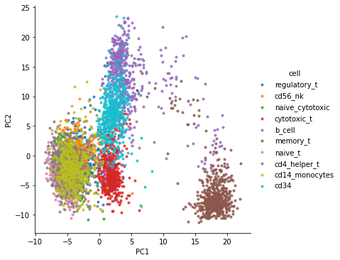
df = pd.DataFrame({ 'PC1' : PC[:,0], 'PC2' : PC[:,1], 'cell' : labels})
df.head()
[10]:
| PC1 | PC2 | cell | |
|---|---|---|---|
| 0 | -1.491188 | 2.378841 | regulatory_t |
| 1 | -1.394000 | -5.895192 | regulatory_t |
| 2 | -2.681231 | -1.834112 | regulatory_t |
| 3 | 1.455147 | 0.239732 | regulatory_t |
| 4 | -0.864700 | -1.447870 | regulatory_t |
[11]:
sns.lmplot(x="PC1", y="PC2", data=df, hue="cell", fit_reg=False, legend=True, markers=".")
plt.show()
[12]:
%%time

# tSNEの計算
model = TSNE(n_components=2, perplexity=20, n_iter=5000, verbose=1, random_state=0)
tsne = model.fit_transform(PC[:,0:9])
[t-SNE] Computing 61 nearest neighbors...
[t-SNE] Indexed 5000 samples in 0.020s...
[t-SNE] Computed neighbors for 5000 samples in 0.291s...
[t-SNE] Computed conditional probabilities for sample 1000 / 5000
[t-SNE] Computed conditional probabilities for sample 2000 / 5000
[t-SNE] Computed conditional probabilities for sample 3000 / 5000
[t-SNE] Computed conditional probabilities for sample 4000 / 5000
[t-SNE] Computed conditional probabilities for sample 5000 / 5000
[t-SNE] Mean sigma: 1.502542
[t-SNE] KL divergence after 250 iterations with early exaggeration: 74.670425
[t-SNE] KL divergence after 5000 iterations: 1.360592
CPU times: user 5min 29s, sys: 1.88 s, total: 5min 31s
Wall time: 2min 49s
[14]:
df = pd.DataFrame({ 'tSNE_1' : tsne[:,0], 'tSNE_2' : tsne[:,1], 'cell' : labels})
df.head()
[14]:
| tSNE_1 | tSNE_2 | cell | |
|---|---|---|---|
| 0 | 29.867262 | -35.284283 | regulatory_t |
| 1 | -6.607394 | -20.787622 | regulatory_t |
| 2 | 21.704603 | -10.506199 | regulatory_t |
| 3 | 28.161837 | -41.953533 | regulatory_t |
| 4 | 24.546949 | -39.936260 | regulatory_t |
[15]:
sns.lmplot(x="tSNE_1", y="tSNE_2", data=df, hue="cell", fit_reg=False, legend=True, markers=".")
plt.show()

[17]:
# UMAPの計算
# UMAPが入っていない場合は以下のコマンドでインストール
!pip install umap-learn
Collecting umap-learn
  Downloading https://files.pythonhosted.org/packages/75/69/85e7f950bb75792ad5d666d86c5f3e62eedbb942848e7e3126513af9999c/umap-learn-0.5.1.tar.gz (80kB)
     |████████████████████████████████| 81kB 3.5MB/s
Requirement already satisfied: numpy>=1.17 in /usr/local/lib/python3.7/dist-packages (from umap-learn) (1.19.5)
Requirement already satisfied: scikit-learn>=0.22 in /usr/local/lib/python3.7/dist-packages (from umap-learn) (0.22.2.post1)
Requirement already satisfied: scipy>=1.0 in /usr/local/lib/python3.7/dist-packages (from umap-learn) (1.4.1)
Requirement already satisfied: numba>=0.49 in /usr/local/lib/python3.7/dist-packages (from umap-learn) (0.51.2)
Collecting pynndescent>=0.5
  Downloading https://files.pythonhosted.org/packages/af/65/8189298dd3a05bbad716ee8e249764ff8800e365d8dc652ad2192ca01b4a/pynndescent-0.5.2.tar.gz (1.1MB)
     |████████████████████████████████| 1.2MB 7.8MB/s
Requirement already satisfied: joblib>=0.11 in /usr/local/lib/python3.7/dist-packages (from scikit-learn>=0.22->umap-learn) (1.0.1)
Requirement already satisfied: llvmlite<0.35,>=0.34.0.dev0 in /usr/local/lib/python3.7/dist-packages (from numba>=0.49->umap-learn) (0.34.0)
Requirement already satisfied: setuptools in /usr/local/lib/python3.7/dist-packages (from numba>=0.49->umap-learn) (56.0.0)
Building wheels for collected packages: umap-learn, pynndescent
  Building wheel for umap-learn (setup.py) ... done
  Created wheel for umap-learn: filename=umap_learn-0.5.1-cp37-none-any.whl size=76569 sha256=c09e08d6ed4eb7bc3b9c7820dd24fddafa346ae81016b8f38141d12de874e7dd
  Stored in directory: /root/.cache/pip/wheels/ad/df/d5/a3691296ff779f25cd1cf415a3af954b987fb53111e3392cf4
  Building wheel for pynndescent (setup.py) ... done
  Created wheel for pynndescent: filename=pynndescent-0.5.2-cp37-none-any.whl size=51351 sha256=d985da65f48b7dfa7477edfea356573c168435e20c3e5bd503aa1e796bf6a0f0
  Stored in directory: /root/.cache/pip/wheels/ba/52/4e/4c28d04d144a28f89e2575fb63628df6e6d49b56c5ddd0c74e
Successfully built umap-learn pynndescent
Installing collected packages: pynndescent, umap-learn
Successfully installed pynndescent-0.5.2 umap-learn-0.5.1
[18]:
import umap
um = umap.UMAP().fit_transform(PC[:,0:9])
[19]:
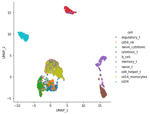
df = pd.DataFrame({ 'UMAP_1' : um[:,0], 'UMAP_2' : um[:,1], 'cell' : labels})
df.head()
[19]:
| UMAP_1 | UMAP_2 | cell | |
|---|---|---|---|
| 0 | 1.409212 | -2.458809 | regulatory_t |
| 1 | -0.491749 | -1.008856 | regulatory_t |
| 2 | 0.097904 | -2.531204 | regulatory_t |
| 3 | 1.619742 | -2.151538 | regulatory_t |
| 4 | 1.497223 | -2.088444 | regulatory_t |
[20]:
sns.lmplot(x="UMAP_1", y="UMAP_2", data=df, hue="cell", fit_reg=False, legend=True, markers=".")
plt.show()
2.6. まとめ
PCA, tSNE, UMAP程度であれば特別な1細胞解析用ツールを使わずともこのように簡単に計算・図示できます。 一方、フィルタリングや正規化などは独自のプロトコルが採用されていることが多いので、そういった点に関しては専用のツールを使う方がよいでしょう。
[22]:
!pip install sinfo
Collecting sinfo
  Downloading https://files.pythonhosted.org/packages/e1/4c/aef8456284f1a1c3645b938d9ca72388c9c4878e6e67b8a349c7d22fac78/sinfo-0.3.1.tar.gz
Collecting stdlib_list
  Downloading https://files.pythonhosted.org/packages/7a/b1/52f59dcf31ead2f0ceff8976288449608d912972b911f55dff712cef5719/stdlib_list-0.8.0-py3-none-any.whl (63kB)
     |████████████████████████████████| 71kB 3.6MB/s
Building wheels for collected packages: sinfo
  Building wheel for sinfo (setup.py) ... done
  Created wheel for sinfo: filename=sinfo-0.3.1-cp37-none-any.whl size=7012 sha256=5f74562827813a1ef0cd449ad4e331b1b3c8f550bbb2c1bbaf203e0897dc5c20
  Stored in directory: /root/.cache/pip/wheels/11/f0/23/347d6d8e59787c2bc272162d18223dc3b45bd6dc40aceee6af
Successfully built sinfo
Installing collected packages: stdlib-list, sinfo
Successfully installed sinfo-0.3.1 stdlib-list-0.8.0
[23]:
from sinfo import sinfo
sinfo()
-----
matplotlib  3.2.2
numpy       1.19.5
pandas      1.1.5
seaborn     0.11.1
sinfo       0.3.1
sklearn     0.22.2.post1
umap        0.5.1
-----
IPython             5.5.0
jupyter_client      5.3.5
jupyter_core        4.7.1
notebook            5.3.1
-----
Python 3.7.10 (default, Feb 20 2021, 21:17:23) [GCC 7.5.0]
Linux-4.19.112+-x86_64-with-Ubuntu-18.04-bionic
2 logical CPU cores, x86_64
-----
Session information updated at 2021-04-30 12:49